TADKit - Interactive Anomaly Detection demonstrator

import os
os.environ["TF_CPP_MIN_LOG_LEVEL"] = "3"

import numpy as np
import pandas as pd
import matplotlib.pyplot as plt

from ouagen import ornstein_uhlenbeck_anomaly


t = np.arange(1000)
t = t / t.shape[0]
pre_X, pre_y = ornstein_uhlenbeck_anomaly(
    t,
    size=20,
    noise_scale=1,
    mean_reverting=3,
    anomaly_freq=.1,
    anomaly_duration=0.005,
    anomaly_scale=40,
)
t = pd.to_datetime('2021-01-01') + pd.Timedelta(1, 'h') * np.arange(t.shape[0])
X = pd.DataFrame(pre_X, index=t, columns=[f'X{i}' for i in range(pre_X.shape[1])])
y = pd.DataFrame(pre_y[:, None], index=t, columns=['y'])
async_X = X.melt(value_vars=X.columns.tolist(), ignore_index=False).rename(
    columns={"variable": "sensor", "value": "data"}
)
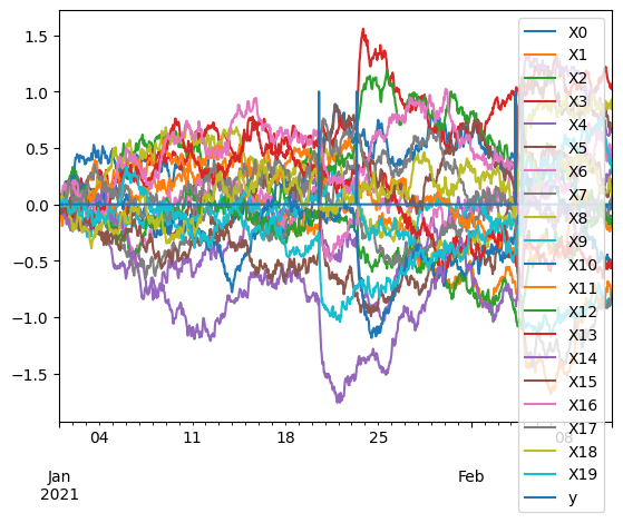
oua = pd.concat([X, y], axis=1)
oua.plot()
# oua.to_csv("oua.csv")

import ipywidgets as widgets

# Create a dropdown selection widget
select = widgets.Dropdown(
    options=["synchronous", "asynchronous"],
    value="synchronous",
    description='Select:'
)
display(select)

from tadkit.catalog.rawtowideformatter import RawToWideFormatter

target_X = X if select.value == "synchronous" else async_X
formatter = RawToWideFormatter(
    data=target_X,
    backend="pandas"
)
print(f"Formatter has {formatter.available_properties=}")

Formatter has formatter.available_properties=['synchronous', 'pandas_backend', 'fixed_time_step']

This allows to select a training interval, a resampling resolution and the set of target sensors for learning.

from query_selection import query_widget_selection

query_dict = query_widget_selection(formatter.query_description)

query_translated = {key: widget.value for key, widget in query_dict.items()}
X_train = formatter.format(**query_translated)
query_translated.pop("target_period")
X_test = formatter.format(**query_translated)

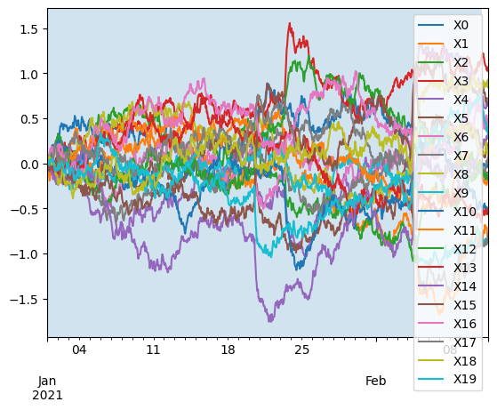
ax = X_test.plot()
ax.axvspan(X_train.index[0], X_train.index[-1], alpha=0.2)
plt.show()

from tadkit.base.registry import registry
import tadkit.catalog.registry_init  # ensure registrations happen

registry.print_catalog_classes()
registry.list_learners()
registry.match_learners(formatter)

[registry] Skipping optional learner 'DataReconstructionAD': No module named 'cnndrad'
[registry] Skipping optional learner 'DiLAnoDetectm': No module named 'sbad_fnn'
[TADkit registered Catalog]
Class learner_name='IsolationForest' is registered in TADKit.
IsolationForest is operational in this environment.
IsolationForest is implicit child of TADLearner.
Class learner_name='KDEOutlierDetector' is registered in TADKit.
KDEOutlierDetector is operational in this environment.
KDEOutlierDetector is implicit child of TADLearner.
Class learner_name='GMMOutlierDetector' is registered in TADKit.
GMMOutlierDetector is operational in this environment.
GMMOutlierDetector is implicit child of TADLearner.
Class learner_name='TopologicalAnomalyDetector' is registered in TADKit.
TopologicalAnomalyDetector is operational in this environment.
TopologicalAnomalyDetector is implicit child of TADLearner.
Class learner_name='KcpLearner' is registered in TADKit.
KcpLearner is operational in this environment.
KcpLearner is implicit child of TADLearner.

[sklearn.ensemble._iforest.IsolationForest,
 tadkit.catalog.sklearners.KDEOutlierDetector,
 tadkit.catalog.sklearners.GMMOutlierDetector,
 tdaad.anomaly_detectors.TopologicalAnomalyDetector,
 kcpdi.kcp_ss_learner.KcpLearner]

for learner_cls in registry.match_learners(formatter):
    learner = learner_cls()  # instantiate directly
    print(f"Instantiated {learner_cls.__name__}")

Instantiated IsolationForest
Instantiated KDEOutlierDetector
Instantiated GMMOutlierDetector
Instantiated TopologicalAnomalyDetector
Instantiated KcpLearner

from tadkit.utils.param_spec import params_from_class
from tadkit.utils.render_widgets_from_params import render_widgets_from_params

learner_params = {}
for learner_class in registry.match_learners(formatter):
    learner_params.setdefault(learner_class.__name__, {})
    print(learner_class.__name__)
    params_specs = params_from_class(learner_class)
    widgets, learner_params[learner_class.__name__] = render_widgets_from_params(params_specs)

IsolationForest

KDEOutlierDetector

GMMOutlierDetector

TopologicalAnomalyDetector

KcpLearner

learner_params["TopologicalAnomalyDetector"]()

{'step': 5,
 'tda_max_dim': 1,
 'contamination': 0.1,
 'n_centers_by_dim': 5,
 'random_state': 42,
 'window_size': 20,
 'support_fraction': None}

learners = {
    learner_class.__name__:
    learner_class(**learner_params[learner_class.__name__]())
    for learner_class in registry.match_learners(formatter)
}
learners

{'IsolationForest': IsolationForest(),
 'KDEOutlierDetector': KDEOutlierDetector(),
 'GMMOutlierDetector': GMMOutlierDetector(),
 'TopologicalAnomalyDetector': TopologicalAnomalyDetector(window_size=20),
 'KcpLearner': KcpLearner()}

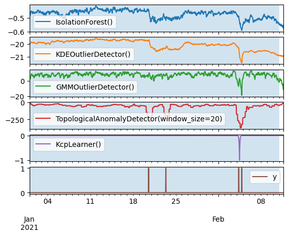
Fit on train query, score on the entire series.

# Fit loop:
anomalies = pd.DataFrame(index=X_test.index)
predictions = pd.DataFrame(index=X_test.index)
for learner_name, learner_object in learners.items():
    print(f"Fitting {learner_name}")
    learner_object.fit(X_train)

# Score loop:
for learner_name, fitted_learner_object in learners.items():
    print(f"Scoring with {learner_name}")
    anom_score = fitted_learner_object.score_samples(X_test)
    anomalies[str(fitted_learner_object)] = anom_score
    predictions[str(fitted_learner_object)] = fitted_learner_object.predict(X_test)

Fitting IsolationForest
Fitting KDEOutlierDetector
Fitting GMMOutlierDetector
Fitting TopologicalAnomalyDetector
Fitting KcpLearner
Scoring with IsolationForest
Scoring with KDEOutlierDetector
Scoring with GMMOutlierDetector
Scoring with TopologicalAnomalyDetector
Scoring with KcpLearner

axes = pd.concat([anomalies, y], axis=1).plot(subplots=True)
[ax.axvspan(X_train.index[0], X_train.index[-1], alpha=0.2) for ax in axes]
plt.show()

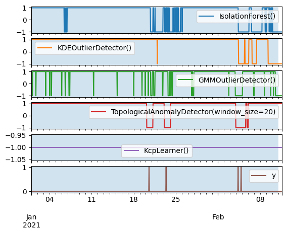
axes = pd.concat([predictions, y], axis=1).plot(subplots=True)
[ax.axvspan(X_train.index[0], X_train.index[-1], alpha=0.2) for ax in axes]
plt.show()

from plotly.offline import init_notebook_mode
from plotly.graph_objs import *
init_notebook_mode(connected=True)         # initiate notebook for offline plot

pd.options.plotting.backend = "plotly"
df = pd.concat([anomalies.apply(lambda x: (x - x.min()) / (x.max() - x.min())), y], axis=1)
import plotly.express as px
fig = df.plot(color_discrete_sequence=px.colors.qualitative.Set2)
fig.update_layout(
    legend=dict(
        orientation="v",
        entrywidth=100,
        yanchor="bottom",
        y=1.02,
        xanchor="right",
        x=1
    ),
    width=1000,
    height=600,
)
fig.show()
pd.options.plotting.backend = "matplotlib"